


WorkloadManagerDemonstration
Overview
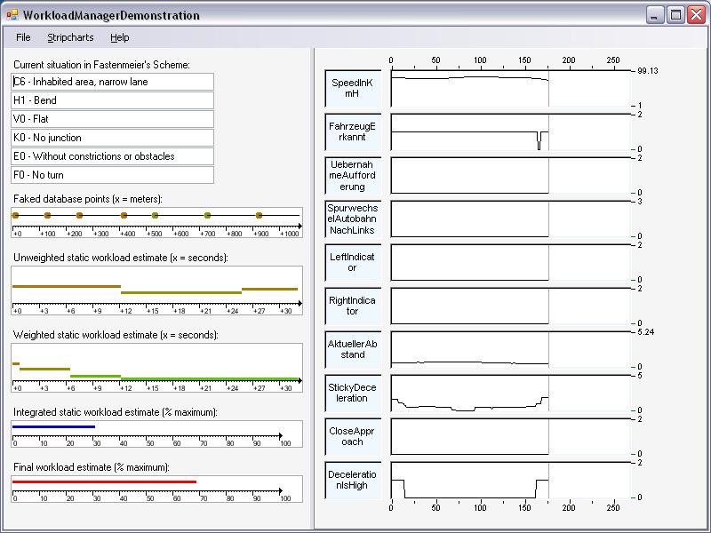
This is an attempt to answer questions about the SANTOS sub-project 'Workload Manager'. I wrote the little demonstration application WorkloadManagerDemonstration that installs with the 'ClickOnce' technique on MS Windows systems. The bootstrapper will install the .NET Framework Version 2 if necessary (Win 95 - Win XP, pre-installed on Vista). If you download and unzip oneofthe36rides.txt you can load it into the demonstration and playback half an hour of real-world workload estimation. It looks like this:
Background
Workload estimation is carried out in a two-stage process. In stage one, a basic estimate is generated by projectively tracking the EDDAS (Extended Databases for Driver Assistance Systems; cf. Schraut, 2000) map to identify the oncoming (statically defined) traffic situations and looking up the respective workload indicators for these situations. In WorkloadManagerDemonstration map-tracking is faked by a semi-random look-ahead into the loaded file. In stage two, this basic estimate is fine-tuned using information about dynamic aspects of the driving situation. WorkloadManagerDemonstration gets this information from the file, the real-world application got it via multicast TCP/IP - 'receivers'.
To be able to track the EDDAS map, the system had to know its exact geographical position. This was achieved using a service based on the global positioning system (GPS) called differential GPS (DGPS). DGPS is a technique used to improve positioning accuracy by determining the positioning error at a known location and subsequently incorporating a corrective factor into the position calculations of DGPS receivers via real-time radio transmission. These DGPS receivers must operate in the same area and simultaneously track the same satellites. Using this technique, positioning error could be reduced to ±3 m or less. DGPS became obsolete in 2001 when Bill Clinton ended the so-called selective availability (a designed corruption of the data).
A map tracking algorithm matched the vehicle position to the EDDAS map and generated a forecast of the route (cf. Schraut, 2000). The accuracy of this projection depends on the level of detail of the digital map and its range depends on the absence of oncoming intersections, as you can never know which route the driver will choose at a junction. However, it is possible to detect whether a driver intends to turn left or right by monitoring the indicator status. Since the driver's route was determined by the experimental procedure of the evaluation experiment indicator status was not used for route prediction in this experiment.
The workload indicator for each situation class is read from a look-up table, thus transforming the sequence of situations into a sequence of workload level projections. The time at which a given point or situation will be reached is anticipated on the basis of the current driving speed. The greater the distance to a point, the more uncertainty lies in this forecast in the time domain, since the assumption that driving speed will remain constant is a coarse simplification. Nevertheless, the fast iteration cycle (10 Hz) of the computations makes the forecast precise enough for situations in the vicinity. One question here is how many situations ahead should be considered, or in other terms, how far an average driver could be expected to look ahead.
Verwey's (2000) guess is that intersections and roundabouts should be assumed to 'begin' 4 s before the situation is actually encountered, in order to take into account the workload caused while approaching these road situations. While this seems plausible, there is no theoretical foundation for this value. I wanted to use the maximum look-ahead distance actually used by drivers. It is known that drivers do lower their driving speeds on motorways on account of reduced visibility conditions in fog when visibility is about 300 m or lower (Hawkins, 1988), so 300 m should be a good estimate. Look-ahead is most relevant when driving at high speeds. On our test route, which does not include highway driving, the maximum legally allowed speed is 100 km/h. At a speed of 100 km/h, a 300 m look-ahead corresponds to 10.8 s time headway, but it is not uncommon and is legally allowed to drive at speeds of 200 km/h and more on German motorways, which reduces the 300 m look-ahead to just about 5 s and less in the time domain. On the basis of these considerations, I derived my own proposal for generic proximity weighting of the workload forecast: The upcoming 5 s are taken into account fully, and then weighting is applied with an exponential first order decay: Weight = 2.71866 * exp(-TimeAheadInSeconds / 4.72657). It should be noted that the decay function is only an 'educated guess', inspired by the idea that the importance of remote situations is diminishing. The time-integrated value of the weighted workload forecasts is used as the basic workload estimate. I tried to show you a symbolic visualization of these steps in WorkloadManagerDemonstration.
This basic workload estimate, which depends only on the situations ahead, is refined using knowledge about dynamic aspects of the traffic environment and variables of vehicle dynamics which are indicative of critical driving manoeuvres. These refinements are (C pseudo code):
// refine strain estimation and quality with dynamic traffic situation information

if (pSa2Si->AccOnline) // should alway be true
{
    if (pSa2Si->FahrzeugErkannt) // leading vehicle detected
    {
        // if nothing special happens, complexity is only slightly increased
        GloSit2Santos.Komplexitaetsgrad *= COMPLEXITY_REWEIGHTFACTOR_IF_FZGERKANNT;

        // derived from Weinberger's study, p 121
        bApproachDetector = WeightDistWeinberger(GloSit2Santos.Komplexitaetsgrad,pSa2Si->AktuellerAbstand);
    }

    // It means also stress if there are red traffic lights ahead within a look-ahead
    // of about 50 meters (experience from URE Experiment, March 2001). We can detect
    // traffic lights ahead from the FDK Santos5 value, but we do know nothing about
    // signal state. So we assume a probability of 0.5 that we have red light
    // (this uncertainty is reflected in the quality value).
    // Note: this rule never fired because there were no traffic lights on the test track
    if (PossiblyRedLightsInNext5Seconds())
    {
        GloSit2Santos.Komplexitaetsgrad *= COMPLEXITY_REWEIGHTFACTOR_NEARAMPEL;
        GloSit2Santos.Qualitaet = 0.5;
    }

    // detect extreme negtive acceleration from speed history
    if (bApproachDetector == false) // otherwise we already have a better guess
    {
        bBreakDetector = WeightHeavyBreaking(GloSit2Santos.Komplexitaetsgrad,PrRe.dftStickyDeceleration);
    }

    if (pSa2Si->UebernahmeAufforderung) // ACC commits control back to the driver
    {
        // this event's complexity should override the normal estimation
        // (experience from URE Experiment, March 2001)
        GloSit2Santos.Komplexitaetsgrad = COMPLEXITY_OF_UEBERNAHMEAUFFORDERUNG;
        GloSit2Santos.Qualitaet = .95;
    }
}

if (bApproachDetector == false) // otherwise we already have a better guess
{
    // remark: fzd's criterion is speed > 70 km/h this can also happen on other roads than BAB
    if (pSa2Si->SpurwechselAutobahnNachLinks) // lane change detected
    {
        GloSit2Santos.Komplexitaetsgrad *= COMPLEXITY_REWEIGHTFACTOR_UEBERHOLEN;
        GloSit2Santos.Qualitaet = .80;
    }
    // yet another overtaking detector
    else if (IsLeftIndicatorOn(pSa2Si->Blinker) && NoCrossingInNext10Seconds())
    {
        GloSit2Santos.Komplexitaetsgrad *= COMPLEXITY_REWEIGHTFACTOR_UEBERHOLEN;
        GloSit2Santos.Qualitaet = .80;
        pSa2Si->SpurwechselAutobahnNachLinks = TRUE;
    }
}

// slight correction of weightings using environmental information

// nighttime driving has the smallest effect
// Note: this rule never fired because because we did not test at nighttime
if (pSa2Si->Helligkeit.Enum & SITR_Helligkeit::SITR_HL_DUNKEL) // sensor says: it's dark
{
    GloSit2Santos.Komplexitaetsgrad *= COMPLEXITY_REWEIGHTFACTOR_NIGHTTIME;
    GloSit2Santos.Qualitaet += .025; // next to nothing better
}

// rain has an effect if it is heavy rain (sensor definition is crucial)
// Note: this rule never fired because August 2001 was a very dry month
if (pSa2Si->Regensenor.Enum & SITR_Regensensor::SITR_RS_REGEN) // sensor says: it's raining
{
    GloSit2Santos.Komplexitaetsgrad *= COMPLEXITY_REWEIGHTFACTOR_RAINING;
    GloSit2Santos.Qualitaet += .025; // next to nothing better
}

// road surface condition has a moderate effect
// Note: this rule never fired because August 2001 was a very dry month
if (pSa2Si->Reibwert.Enum & SITR_Reibwert::SITR_RW_NASS) // sensor says: road is wet
{
    GloSit2Santos.Komplexitaetsgrad *= COMPLEXITY_REWEIGHTFACTOR_WETROAD;
    GloSit2Santos.Qualitaet += .025; // next to nothing better
}

// slippery road should have more effect
// Note: this rule never fired because August 2001 was a very dry month
if (pSa2Si->Reibwert.Enum & SITR_Reibwert::SITR_RW_GLATT) // sensor says: road is slippery
{
    GloSit2Santos.Komplexitaetsgrad *= COMPLEXITY_REWEIGHTFACTOR_SLIPPERYROAD;
    GloSit2Santos.Qualitaet += .025; // next to nothing better
}

// ceilings are a 1.0
if (GloSit2Santos.Qualitaet > 1.)
{
    GloSit2Santos.Qualitaet = 1.;
}

if (GloSit2Santos.Komplexitaetsgrad > 1.)
{
    GloSit2Santos.Komplexitaetsgrad = 1.;
}
Definitions of the detectors are:
// Approaching another vehicle means high strain, Weinberger p 121.
// We set strain at 1 sec follow dist equal to COMPLEXITY_OF_UEBRNAHMEAUFFORDERUNG or more
// and we assume that the strain will increase linear from where it would be without
// taking critical distance into account. These settings are results of hands-on
// experience and fine-tuning of the workload estimator. Do not change them without
// practical experience.
bool WeightDistWeinberger(double& dftStrain2Weight, double secdist)
{
    static double dftLastSecDist = 0.;
    double dftDiffToLast = secdist - dftLastSecDist;

    if (secdist <= 0.) // invalid, no leading vehicle or error
    {
        return false;
    }
    else if (secdist < 3. && dftDiffToLast < -0.2) // driver will have to decide whether to take control or not
    {
        dftStrain2Weight += COMPLEXITY_OF_UEBERNAHMEAUFFORDERUNG / secdist;
        dftLastSecDist = secdist;
        returntrue;
    }

    dftLastSecDist = secdist;
    return false;
}

// from Weinberger results p 123 it can be argued, that accelerations
// smaller -1 m/s^2 (i.e. heavy breaking) should be a good driver
// strain detector. Note that DftHistoryOfSpeeds[] contains the speed history
// in m/s and not in km/h. Here we implement an after-effect of breaking, by
// looking at the speed history i.e. the effect of breaking is somewhat 'sticky'.
bool WeightHeavyBreaking(double& dftStrain2Weight, double& deceleration)
{
    const double maxFeasibleDeceleration = 5.; // in m/s^2 (Becker, 1995, Weinberger, 2000)
    double speedDiffs[HISTORYSLOTS-1];

    for (int i = 1; i < HISTORYSLOTS; i++)
    {
        speedDiffs[i-1] = DftHistoryOfSpeeds[i] - DftHistoryOfSpeeds[i-1];
    }

    // look for peak deceleration in the near history
    double maximum = 0.;

    for (i = 0; i < HISTORYSLOTS - 1; i++)
    {
        if (speedDiffs[i] > maximum)
        {
            maximum = speedDiffs[i];
        }
    }

    // because we are called with 10 Hz, maximum reflects deceleration
    // in m/100msec^2, hence:
    deceleration = maximum * 10.; // should result in m/s^2

    if (deceleration > maxFeasibleDeceleration) // impossible, must be measurement error
    {
        deceleration = maxFeasibleDeceleration;
    }

    if (deceleration > 1.) // Weinberger finds this for 4 classes of critical situations
    {
        dftStrain2Weight += COMPLEXITY_OF_UEBERNAHMEAUFFORDERUNG * (deceleration / maxFeasibleDeceleration);
        return true;
    }

    return false;
}

// Note: the array Mp[] contains the oncoming data points
bool NoCrossingInNext10Seconds(void)
{
    bool retVal = true;
    __int16 crossings;

    for (int i = 0; i < METASEQUENCE_LENGTH; i++)
    {
        if (Mp[i].dftReachedInSec > 10.) // too far away in the time domain
        {
            break;
        }
        else
        {
            crossings = Mp[i].rawPunkt.val5;
            crossings >>= 6;
            crossings &= 0x0007;
        }

        if (crossings != GFC_K0)
        {
            retVal = false; // i.e. there is a crossing
            break; // it is already sufficient if we found only one
        }
    }

    return retVal;
}
I distinguished between free driving and following a leading car. As Weinberger (2001) explicated, drivers of ACC vehicles often felt uneasy when they were approaching a slower leading vehicle. This was because in contrast to some early prototypes, the ACC systems which were 'state of the art' in 2001 did not automatically handle every slow-down manoeuvre necessitated by a slower leading vehicle. The maximum deceleration the ACC could request from the brake system was typically limited to about -2 m/s2. This led to situations where the driver had to take over control by pressing the brake pedal (pressing the brake pedal deactivated the ACC). In some situations, it was not perfectly clear whether taking over control would be needed or not, so an ACC-equipped vehicle required some additional attention from the driver when approaching a leading vehicle. Moreover, drivers did wait to see if the ACC would cope with the situation and then reacted later by decelerating rapidly if the system did not recover the time gap sufficiently (Marsden, McDonald, & Brackstone, 2001).
In the course of some informal tests, subjects told us that compared to free driving on an empty road, they subjectively felt a slight increase in workload when following a leading vehicle. However, the subjects felt a considerable increase in workload whenever a close following distance decreased even further. Accordingly, the mere fact of detecting a leading vehicle (the radar sensor had a maximum 'viewing distance' of 120 m) is taken into account by multiplying the basic workload estimate by a factor of 1.1. However, when rapid approaches are detected at a point when time headway amounts to 3 s or less, the workload estimate is incremented considerably at once. The shortest time headways we measured were approximately 0.5 s. The system should not be made too hesitant in responding to rapid approaches, because detection of a close target can occur abruptly, especially in very narrow curves, where the radar system can run into problems because of its limited 'field of view' (8 degrees horizontally).
The distinction I made between free driving, following and rapid approach fits well into the three-phase concept of approaching a leading vehicle proposed by Vogel (2002). In this concept, a free vehicle at first becomes an influenced vehicle at a 6 s time headway and then a following vehicle at a 2–3 s time headway. Based on the analysis of 110,269 headways of following vehicles, Vogel argues that drivers in fact do drive at time headways of between 2 and 3 s, as the correlation between the speed of the leading and the following vehicle lies between approximately .50 and .70 in this time headway interval. But correlations already begin to rise at a 6 s time headway, while they are consistently low at headways greater than 6 s. The threshold of 6 s can therefore be seen as the line of demarcation between driving freely and driving under some influence of the vehicle ahead. This time headway of 6 s corresponds to 83 m at 50 km/h and to 167 m at 100 km/h. It is still unclear whether the 6 s threshold is psychologically salient (Vogel, 2002). Moreover, the 6 s threshold was derived from measurements at an urban junction, so its validity may be restricted to this traffic situation. Therefore, I considered it wise to use the information for a detected leading vehicle at a distance headway of up to 120 m (i.e. the maximum distance detected by the ACC radar) to moderately increase the workload estimate, as the possibility of a slightly premature increase in estimation of the workload is more acceptable than a delayed one.
If a software detector encounters an intersection with traffic lights on the route projected in the time domain within the next 5 s, both arms of the fine tuning logic apply a factor of 1.1, as an approach to such an intersection is considered particularly complicated (Fastenmeier, 1995). The 5 s look-ahead applied here is a slight extension of Verwey's (2000) proposal of 4 s.
If no leading vehicle is detected but the driver hit the brakes hard, I also add a considerable increment to the workload estimate (implemented in procedure WeightHeavyBreaking). Braking hard is defined as a deceleration of more than -1 m/s2. Here, I apply a less extreme increment than that used when a rapid approach is detected by ACC sensor data, as rather hard decelerations may just be the result of a sporty driving style. Nevertheless, the rapid approach and hard braking detectors address similar situations. The approach detector simply captures some situations in advance where the driver may need to brake very soon. While accelerations are never critical manoeuvres in volume production vehicles, extreme decelerations are indicative of situations that induce workload. This can be illustrated by the fact that Weinberger (2001) finds mean decelerations of more than -2 m/s2 in all his critical situations, during which drivers took control and overrode the ACC system.
pSa2Si->UebernahmeAufforderung means that ACC commits control back to the driver. In the demonstrator vehicle, which was used to evaluate the system, optical and acoustical signals prompted the driver to take over the longitudinal vehicle control whenever the ACC-induced deceleration was not sufficient to avoid a crash or when other restrictions applied. For example, the ACC switched itself off if the vehicle's speed became slower than 30 km/h, a situation that typically arises when approaching red traffic lights. The acoustic prompt was useful to beginners, but annoying to experienced ACC drivers, who prefered to switch off the auditory signal. Whether experienced or not, the exact point in time when the driver had to take over control always signified mental strain. On average, subjects judged the amount of 'activation' they felt in these moments to be 92% of an imaginary maximum. As ACC committal (take-over request) is a very distinct occurrence that always induces workload, I set the workload estimate to .92 for the time at which the prompting signals were displayed.
Finally, I have to explain the overtaking detector (pSa2Si->SpurwechselAutobahnNachLinks). Overtaking is defined as a situation when the left indicator is in operation at driving speeds faster than 70 km/h or (else if...) at points on the route where there are no intersections (including T-junctions) in the route projection while applying a look-ahead of 10 s. This conditional weighting begins at the very moment when the radar sensor loses 'sight' of the leading vehicle, i.e. when overtaking is actually in progress. The factor of 1.44 applied to the workload estimate in these moments corresponds to the reduction in secondary task glances whilst overtaking that we found during the analysis of overtaking situations from a pilot study.
Whenever the finely tuned workload estimate exceeded a threshold value, incoming telephone calls were redirected to the mailbox, instead of signalling them to the driver. This was what we carried out for the purpose of evaluation in the demonstrator car. Of course, it is possible to 'silence' short messages, email, and additional displays of all kind in the same way.
I used a threshold value of .35 for the evaluation experiment, because it was necessary to 'sensitise' the workload estimator to a sufficient degree in order to be able to suppress a considerable amount of incoming telephone calls on the test route. A somewhat higher threshold would have to be applied in a real-life situation. I think, the driver should be allowed to set the threshold, if he wants to.
References
Fastenmeier, W. (1995). Die Verkehrssituation als Analyseeinheit im Verkehrssystem. In W. Fastenmeier (Ed.), Autofahrer und Verkehrssituation: neue Wege zur Bewertung von Sicherheit und Zuverl€aassigkeit moderner Sraßenverkehrssysteme (pp. 27–78). Köln: Verl. TÜV Rheinland.
Hawkins, R. K. (1988). Motorway traffic behaviour in reduced visibility conditions. In A. G. Gale (Ed.), Vision in vehicles II (pp. 9–18). Amsterdam: Elsevier.
Marsden, G., McDonald, M., & Brackstone, M. (2001). Towards an understanding of adaptive cruise control. Transportation Research Part C, 9, 33–51
Schraut, M. P. (2000). Umgebungserfassung auf Basis lernender digitaler Karten zur vorausschauenden Konditionierung von Fahrerassistenzsystemen. Doctoral thesis. [On-line] available: tumb1.biblio.tu-muenchen.de/publ/diss/ei/2000/ schraut.html.
Verwey, W. B. (2000). On-line driver workload estimation. Effects of road situation and age on secondary task measures. Ergonomics, 43, 187–209
Vogel, K. (2002). What characterizes a 'free vehicle' in an urban area. Transportation Research Part F, 5, 313–327
Weinberger, M. (2001). Der Einfluß von Adaptive Cruise Control auf das Fahrerverhalten. Aachen: Shaker.

